| Overview |
| Gravity Loads |
| Lateral Loads |
| Non-Graphical Methods |
|
Powerpoint Illustration (2 MB) |
| Homework Problems |
| Report Errors or Make Suggestions |
Section TA.2
Tributary Areas for Gravity Loads
Last Revised: 08/20/2024
If the beam is supporting a floor, roof, or wall that has a pressure loading normal to the surface, the total force on the beam equals the area of surface supported (i.e. the tributary area) times the pressure on the surface.
Consider a series of floor joists (repetitive beam members) supporting a floor system as shown in the framing plan in Figure TA.2.1.
Figure TA.2.1
Sample Floor Framing System
Taking a closer look at a single joist, as shown in Figure TA.2.2, you can see that the floor system spans as a continuous beam across evenly spaced supports. Note that the floor spans from joist to joist instead of in the same direction as the joist since the floor is substantially stiffer (try the deflection calcs if you want!) in the short direction. In this situation, the floor system will transfer half of a span's uniformly distributed load to the joist on either end of the floor span. So, it can be said that the joist supports all the load on the area shown (the hatched area). Each joist in the system will likewise support the floor system, so that all of the floor area is accounted for.
Figure TA.2.2
Floor Joist Tributary Area
The hatched area is referred to as the tributary area for the joist. It's dimension transverse to the joist is half the distance to the next joist on either side (also known as the tributary width) and it's length is the length of the joist. The total load (in force units) on the joist equals the tributary area (area units) times the uniform pressure loading (force per unit area).
The two dimensional loading diagram is constructed by multiplying tributary width (length units) by the uniform pressure loading (force per unit area) to get the distributed load magnitude (force per unit length of joist). This can be expressed mathematically as:
w = q tw
where:
- w = magnitude of the distributed load (force per unit length)
- q = the magnitude of the uniform load (force per unit area)
- tw = the tributary width (length).
Note that tw = s if the joist spacing is uniform.
Another way to look at this is to consider w to be a representative unit length of the joist. The area that it supports equals the tributary width times the unit length. The load w that that unit length supports equals the tributary area (1*tw) times the uniform pressure load q. Hence the load per that unit length is w = 1*tw*q = q tw.
The idealized beam loading diagram is shown in Figure TA.2.3.
Figure TA.2.3
Idealized Beam Loading Diagram
Noticing that each joist transfers half of its load to each supporting member (i.e. the reactions each equal wL/2), we can now draw the loading diagram for one of the supporting girders.
As the girder collects the joist reactions, we can draw the girder load diagram as having a series of point loads. Figure TA.2.4 shows such a case for a typical girder supporting evenly spaced joist reactions of equal magnitude.
Figure TA.2.4
Girder Loading Diagram
In order to do the analysis we need to have designed the joists so that we know where each joist is located.
To side track for a moment, consider the possibility that we could approximate the series of point loads by an equivalent distributed load. The equivalent distributed load could be computed by
- adding up all the point loads and dividing by the girder length, or
- dividing a point load, P, by the point load spacing, S.
You will get the same answer either way if the reactions are equal and the spacings are equal.
Since we are designing beams for shear, moment, and deflection, approximating the series of point loads as a uniform load will only work if the values for shear, moment and deflection are nearly the same or greater than the values obtained from an analysis of a series of point loads. Let's check this out.
Consider a beam of length L, that supports a series of point loads of magnitude P.
The next three figures compare the results for shear and moment from analysis that consider the loads as point loads and a an equivalent uniform load.
Figure TA.2.5a
Internal Force Comparison when S = L/2
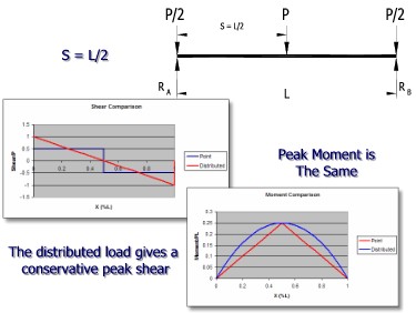
Figure TA.2.5b
Internal Force Comparison when S = L/3
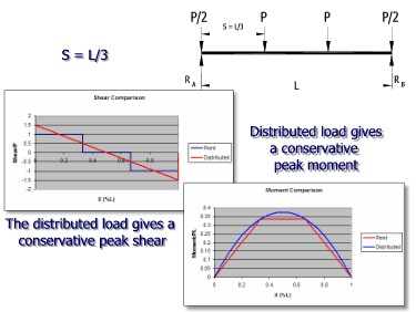
Figure TA.2.5c
Internal Force Comparison when S = L/4
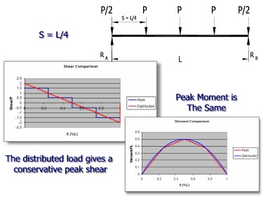
Notice that, as the number of loads increases, the difference between the results for the series of point loads begins to come closer to the uniform load results.
Generally, the approximate method is used whenever the joist spacing is less than or equal to L/4 since the results are pretty close and the uniformly distributed load is easier to analyze than a series of point loads.
So, with the above in mind, lets take a look at one of the girders in Figure TA.2.1. We'll start with the girder on grid line 1 between grids A and B. Instead of computing the joist reactions, we can see that each joist deposits half its load on each of the supporting girder. Therefore, since the floor pressure is uniform, we can say that the girder supports the sum of half the areas of each of the joists. Graphically, we can draw a line down the center of each supported joist and say that all the area between the line and the girder is tributary to the girder. You can see this in Figure TA.2.6. The distance of the tributary area in the direction of the joists is the tributary width.
Figure TA.2.6
Area Tributary to Girder 1,AB
The load diagram for the beam would be that of a simply supported, uniformly loaded beam having a load intensity:
w = q tw
Where tw, in this case is seven (7) feet. Notice that the other girder on grid 1 has the same load intensity. You should be able to say way that is so at this point.
We can repeat this exercise for all the girder in the framing plan. Note that all the floor area must be accounted for! See Figure TA.2.7 to the tributary area assignments for all the girders.
Figure TA.2.7
Girder Tributary Areas
Click on image for Powerpoint animation
Click on the Figure to get a powerpoint animation that dynamically illustrates the girder tributary areas.
Next we look at the columns.
Each column supports either one or two, simply supported, uniformly loaded girders. Each girder adds half it's supported load to each supporting column. Hence, each column supports half the area supported by each contributing girder.
For example, Figure TA.2.8 shows the area tributary to the column at the intersection of grids 1 & B. This area represents half the area supported by girder 1,AB and half the area supported by girder 1,BC.
Figure TA.2.8
Column 1B Tributary Area
As all the load on the floor system is supported by the nine columns, we can draw a diagram illustrating the areas that are tributary to each column. Again... all the area must be accounted for and no part of the area is to be counted twice. Figure TA.2.9 shows the diagram for area tributary to the columns. You can click on the figure to see a powerpoint animation of the areas.
Figure TA.2.9
Column Tributary Areas
Click on image for Powerpoint animation
The load on each column can be determined by multiplying the Tributary Area for each column by the uniform load intensity, q.
Hopefully, you are starting to see the usefulness of this method. You can determine the load on any member of this floor framing plan in any order! Also the analysis of the girders is somewhat simplified.
Now, lets look at a few more challenging framing layouts.
Framing that is not perpendicular to the supported member
A rather common situation is the one illustrated in Figure TA.2.10. In this layout, some of the framing is perpendicular to it's supports and others are not.
Figure TA.2.10
Floor Framing Plan
Click on image for Powerpoint animation
Each joist has the same uniform load intensity, w = q s, but has a different length. The designer will need to decide whether to design for the worst case and use the same for all joists or decrease the size as the joists get shorter.
To find the loading on the two girders, we can readily identify their tributary areas as being half that supported by each joist, so we can draw a line down the center of the joists to divide the two tributary areas as shown in Figure TA.2.11.
Figure TA.2.11
Areas Tributary to the Girders
In this case, if you are observant, you will notice that each girder supports half of all the joists which support all the floor, so it follows that each girder supports half the total floor load. The question now is: How is applied to each girder?
Let's start with girder AB.
In this case the joists are perpendicular to the girder. Each joist reaction can be distributed over a length of girder equal to the joist spacing, s. This means that the linear load intensity is greater at the "A" end of the girder. The 2D load intensity, w, at the A end of the girder equals:
wA = q tw = q (L1/2)
The load intensity at the "B" end of the girder equals zero since tw is zero at this point. The resulting beam load diagram (not including beam self weight) is shown in Figure TA.2.12. If beam self weight is to be included then a uniform load equal to the beam weight per unit length should be added to the loading.
Figure TA.2.12
Girder AB Load Diagram
Another way to arrive at the value for wA is to recognize that the distribution is linearly varying from zero then solve the following triangle equation for wA:
q (Trib. Area) = 0.5 L2 wA
The total load from the diagram equals the tributary area times the load intensity.
Another thing to note is that the load diagram follows the shape of the tributary area diagram in this case. This is always true when the supported framing is perpendicular to the member. This is not precisely true for other situations, as we will now see.
Consider girder BC. In this case the supported framing is not perpendicular to the girder.
A common mistake here is to assume that peak load in the loading diagram occurs where a line perpendicular to the girder passes through the center of the longest joist. This in not right! Note that the longest joist (and the most heavily loaded) transfers all it's load to the "C" end of the girder, making that the largest load intensity. Since joist length's vary linearly, the resulting beam loading diagram is of the same shape as beam loading diagram for girder AB.
As seen in Figure TA.2.13, a joist that is coming into the girder at an angle q from perpendicular spreads it's load over a length s/cos q of the girder. The load intensity per unit length of girder then becomes:
wj = [q*(s (Lj/2))] / [s / cos q] = 0.5 q Lj cos q
where:
- (s (Lj/2)) = the tributary area of the joist that is supported by the girder
- s / cos q = the length of girder over which the joist reaction is distributed.
Figure TA.2.13
Load from a Joist
From this derivation, we can conclude that the load intensity at "C" end of the girder equals
wC = 0.5 q L1 cos q
Alternately, you can find wC by recognizing that the load on the girder has a triangular distribution and then set up the expression that equates the tributary load to the shape of the load diagram:
q (Trib. Area) = 0.5 sqrt (L12 + L22) wC
This results in the load diagram given in Figure TA.2.14.
Figure TA.2.14
Load Diagram for Girder BC
Now let's consider the three columns.
Each column supports one or two ends of the girders. Unfortunately the girders are not uniformly loaded so we cannot say that the girders transfer half their load to each column. When we add it the uniform weight of the beams we get load diagrams of the general shape shown in Figure TA.2.15.
Figure TA.2.15
General Loading Diagram for Girders AB & BC
Since we now have a member with a non-uniform load, we need to actually compute the reactions for the girders then apply them to the columns. The tributary area method is not very useful for these columns in this case.
Note, however, that if the beam self weight is ignored and W2 = 0, then you can say that the reaction at "A" is 2/3 of the total load and the reaction at "B" is 1/3 of the total load on the girder. With uniform pressure, the column at the "A" end can be said to support 2/3 of the beam's tributary area and the "B" end supports 1/3 the beam's tributary area. In the case of the floor system in Figure TA.2.10, this means that each column supports 1/3 of the total floor area.
To see a powerpoint animation that highlights different tributary areas for this problem, click here.
Trial Problems
You can download a PDF file of the various floor configurations shown in Figure TA.2.16. Try your hand at identifying the tributary areas and drawing the loading diagrams for the various girders. Where it is convient to use the tributary area method, identify the areas tributary to the columns and walls that support the joists and girders.
If you have difficulty, take the problems to your instructor for personalized assistance.
Figure TA.2.16
Sample Framing Plans
Click here for PDF of this
Figure