|
|
Section 9.3
Second-Order Effects
Last Revised: 04/19/2021
When an axial compressive force simultaneously occurs with bending, it creates additional bending in the member, causing the internal bending moments to be larger than are predicted using typical first-order structural analysis on the undeflected structure. The magnitude of the increased moment is a function of the applied forces and the stiffness of the chosen member. Design of a structural element subjected to combined axial compression and bending must consider the increased moment in order to provide a member of sufficient strength.
When an axial tension force simultaneously occurs with bending, the resulting bending moment in the member is reduced. As this is a conservative case, the effect is generally ignored and the first-order moments are used in design without modification.
The Mechanics of Second Order Effects
To understand the second-order effects of combined axial compression and bending, consider the beam shown in Figure 9.3.1.
When bending forces are present in a member, there is displacement from the initial longitudinal axis of the member as seen in Figure 9.3.1(a).
Figure 9.3.1
second-order Effects on Bending
Click on image for larger view
Figure 9.3.1(b) is a partial FBD of a portion of the beam that illustrates the deflected shape and internal moment. Shear is ignored for this discussion since it has no effect on the process being described.
In Figure 9.3.1(c) an axial force is added to the member and is shown on the FBD. The presence of the axial force now creates an incremental increase in the internal moment that originally was computed for the undeflected member. The incremental moment increase equals the axial force times the initial deflection = PD1.
The incremental moment increase will, in turn create an incremental increase in deflection, D2, causing the total deflection to equal D1 + D2 as seen in Figure 9.3.1(d).
The cycle will continue as each incremental moment increase creates an incremental increase deflection until either the calculation becomes unstable, or the process converges (i.e., the incremental increases in moment and deflection approach zero). Figure 9.3.1(e) shows the situation where convergence is obtained after n cycles.
A sample second-order analysis for a simple cantilever column with an axial force and applied end moment can be down loaded by clicking here: 2ndOrderAnalysisExample.pdf. The sample second-order analysis is for demonstration purposes only as some simplifying assumptions have been made in the process.
Determining the final internal moment requires either an iterative solution (similar to the one presented above) or a differential equation solution that can be found in other structural engineering texts.
The end result of any of the analysis processes is that the internal moment is larger than the moment predicted by normally used first-order (i.e., equilibrium on the undeflected shape) analysis. It is important that the increased moment (some times referred to as a "magnified" moment) be used when comparing required strength to actual strength. Failure to do so is non-conservative.
Note that each member has two principle axes. The second-order effects can be considered independently to find the magnified moment about each axis.
Member bending and column stiffness have a major impact on the magnitude of the magnified moments. The stiffness of the member is a function of its section properties (Ix and Iy) and material (E) as well as the member support conditions. The values for Ix, Iy, and E are readily determined from the member selected and the material that it is made from. When using the Effective Length or First-Order Analysis methods of analysis, determining the support member conditions often takes a bit more effort and will require an understanding of how the member fits into the finished structure.
SCM Requirements of Required Strengths
The internal forces (i.e., required strengths) used in the SCM equations for combined loading found in SCM H must include second-order effects as well as the other effects outlined in SCM C1. SCM page 2-13 has a good discussion comparing the three available methods for analyzing a structure. For the Direct Analysis and Effective Length methods, second-order effects can be addressed either with a computer program which does second-order analysis or by using the SCM Appendix 8 B1-B2 method. For the First-Order Analysis method second-order effects are "captured through application of an additional lateral load..."
SCM Appendix 8 presents an approach using approximate equations to account for second-order effects on the results of first-order analysis. This approach is suitable for many problems (it was the primary method used prior to the SCM 14th edition) where first-order analysis is reasonably accomplished. With the advent of structural analysis programs which perform iterative second-order analysis, it is possible to obtain the required strengths without using SCM Appendix 8.
First-Order Analysis for use with SCM Appendix 8 Modifiers
When performing a first-order structural analysis, it is necessary to incorporate the requirements of SCM C and SCM Appendix 7. The requirements include--among other things--additional loads and, in some cases, reduced member stiffnesses.
The first major concern is to consider member support conditions. It is necessary to determine if the member under consideration is "braced" or "unbraced". The location of maximum deflection, and hence the magnitude of the second-order effects, are different in each case. Figure 9.3.2 illustrates typical deflected shapes of (a) a braced frame and (b) an unbraced frame. Note the different locations of maximum deflections. The nature of the end conditions will also be important to determining the buckling slenderness of the member.
Figure 9.3.2
Braced vs. Unbraced Columns
Click on image for larger view
Note that the SCM (SCM Appendix 7 commentary) refers to axial force members in braced frames as being "sidesway inhibited" while the same members in unbraced frames as being "sidesway uninhibited".
Also, for an axial force member in a braced building frame, the deflection, d, between the ends of the member is predominate and independent of other members in the same level (i.e., between floor levels where their end points are all connected together by framing and a floor or roof system). In an unbraced building frame, the predominate deflection is the relative lateral joint translation of the two ends, D. Since each end is connected to a floor or roof system, no column can displace laterally unless all other columns in the same level displace equally. Consequently, a lateral deflection, D, in an unbraced frame member is a function of all the other members resisting the deflection in the same level.
In Figure 9.3.3, it can be seen that the columns between the roof and second floor do not have significant lateral joint translation IN THE PLANE SHOWN because of the brace. Consequently, there is little, or no, moment induced in the columns as the result of the lateral loading. The column moments result from eccentrically applied beam reactions, moments from any continuity in the connections and unbalanced loading, or from laterally applied loads to the member itself. The deflections creating the second-order effects are along the length of the member and the relative lateral displacement of the ends is near zero. The displacements in a column are predominately the result of the moments that column sees as opposed to moment due to frame lateral translation.
Figure 9.3.3
Effects of Bracing
Click on image for larger view
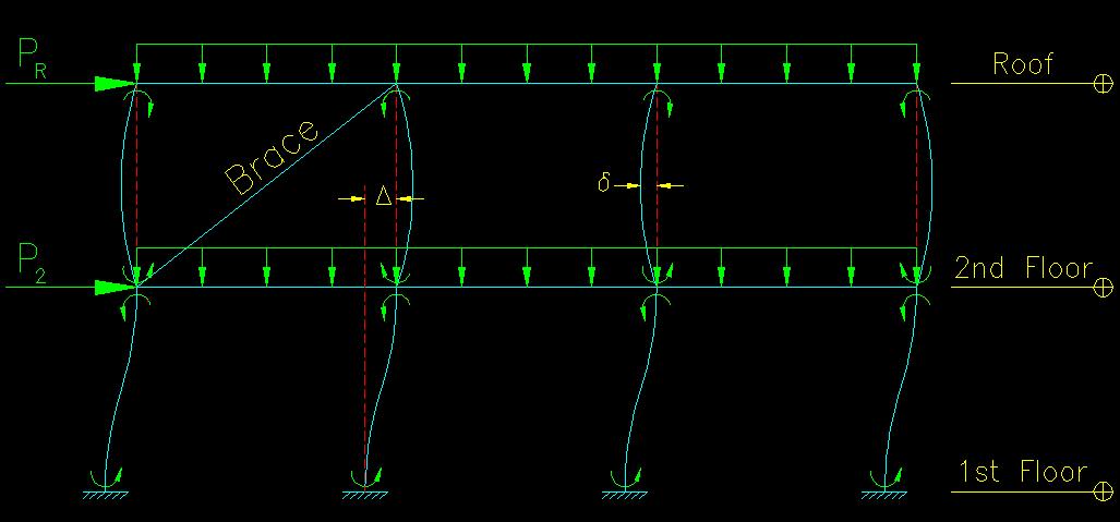
For the columns between the first and second floors, the predominate displacements are caused by the lateral forces applied to the building that cause lateral displacement in the frame and are a function of the stiffness of all the columns in the level that are contributing to the resistance of lateral displacement IN THE PLANE SHOWN. All of the columns in the level have the same lateral joint displacement, D.
As a result of these two behaviors, the magnification of moments that result from loads that cause lateral joint translation is different than the magnification of moments resulting from loads that don't cause lateral joint translation. The normal approach to computing the magnified moments is to do two separate analyses: one with the structure restrained against lateral translation and one without lateral restraint. Figure 9.3.4 shows a simplistic version of the loadings for the two different analyses.
Figure 9.3.4
Two Load Cases
Click on image for larger view
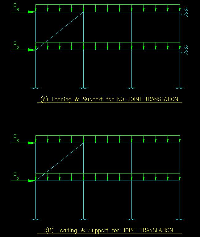
The moments and axial forces from the restrained analysis shown Figure 9.3.4a are then magnified considering no joint translation (in the SCM Appendix 8 these internal forces are labeled Mnt, Pnt). The difference in moments and axial forces from the two analysis represent the moments and axial forces that are the result of joint translation (in the SCM these internal forces are labeled Mlt, Plt). The results are then superimposed to find total moments on each column.
A reasonable approximation for the preliminary design of symmetric frames that are symmetrically loaded can be made by doing an analysis of the structure with just the gravity loads (and without the lateral supports) in order to determine the "nt" internal forces and an analysis with just the lateral loads to determine the "lt" internal forces. This can be done since the gravity loads provide very little "lt" component in such a condition. In most cases, however, these conditions do not exist and two analysis must be performed with the full loading on each with the difference in analysis being that one has lateral restraint and the other does not.
The SCM Appendix 8 approach to determining magnified moments follows the general procedure outlined in this section.
<<< Previous Section <<< >>> Next Section >>>