|
|
Section 4.9
Example Problem 4.4
The example problems presented in this section refer to a spreadsheet solution. Click on the link below to get the file:
Chapter 4: Excel Spreadsheet Solutions
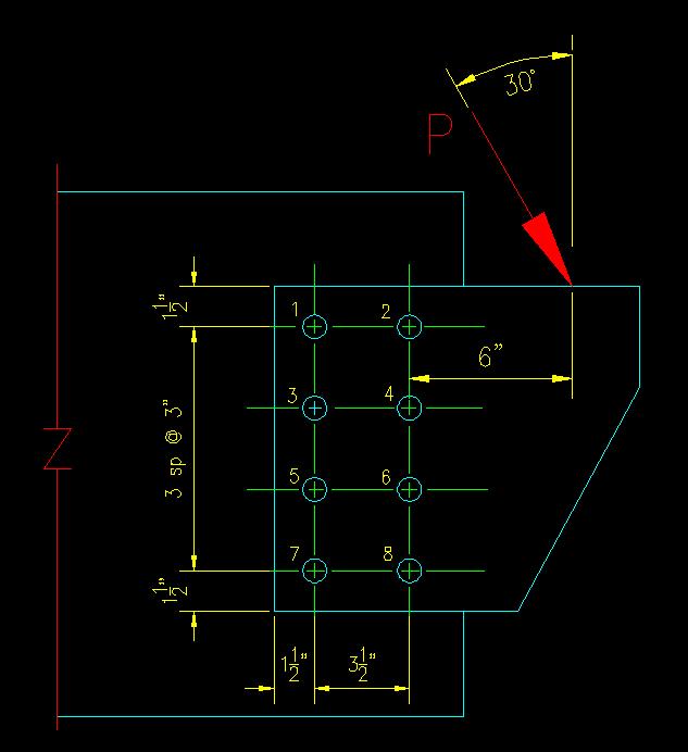
Given: A bracket is connected to a column flange as shown in Figure 4.9.4.1. The bolt information is given on the drawing. Assume that the applied load is 50% D and 50% L. The bolts are fully pretensioned 3/4" dia A490-N bolts in standard holes.
Figure 4.9.4.1
In-Plane Eccentric Load
Click on image for larger view
Wanted: Determine the capacity of the connection based on bolt strength as specified below. Consider both LRFD and ASD. Express your results in terms of service load levels.
- Determine the bearing capacity of the connection using the elastic method.
- Determine the bearing capacity of the connection using the IC method.
Solution:
Determining the bolt capacity is the easiest part of the problem. The difficult part is the analysis to determine the force that each bolt sees. You need to look at the spreadsheet solution for this problem as the following discussion explains what is done in the spreadsheet.
a. Bearing Capacity using Elastic Method
The first task taken is to compute the effective load factors for both LRFD and ASD so that we can convert our answers to a common basis so that they can be compared.
Next the shear rupture (bearing) strength for a single bolt is determined.
The next section includes the given information. Note that a value of 1 kip was used for the applied load. Since we do not know the actual applied load (we have been tasked with determining capacity) and we are computing the coefficient "C" (the relationship between P and rmax) the value used here is irrelevant. A value of 1 is convenient because the result of the analysis is the "C" value.
The eccentricity to the load was determined graphically (in AutoCAD) however, with a bit of trigonometry, the number can be verified.
The force is then moved to the bolt center of gravity (CG), a moment added, and the force is broken into it's horizontal (x) and vertical (y) components.
The first table computes the geometric quantities, c (the distance from the center of each bolt to the CG), and the Ix and Iy contribution of each bolt using the parallel axis theorem (ignoring the Io component because it is small).
The polar moment of inertia, Ip, is the sum of Ix and Iy (as you learned in statics...).
The second table computes the forces in bolts due to each of the three applied forces. The forces are vectorally added to determine the total force in each bolt.
The coefficient C is found to be the ratio of P to rmax. Assuming linear elastic behavior, this coefficient can be used find either P or rmax once the other is known. In this case, we know rmax equals the capacity of a bolt, from there we get the maximum force that can be applied to the joint as shown in the drawings.
b. Bearing Capacity using the IC Method
This approach starts off similar to part (a) of this problem.
Once we get to the analysis, the input data includes the angle of the load, the location of the IC, CG, and point of load application. This data is used to compute the rotation arm, ro, of the applied load about the IC. Knowing the distance between the IC and Load Point and various angles, the law of sines is used to compute ro.
The object of the analysis is to find the location of the IC such that the equilibrium equations are satisfied. This is done by either manually changing the coordinates of the IC or using the "Solver" command in Excel.
The first table computes the distance of each bolt from the IC and determines the deformation in each bolt according the procedure's assumptions.
The second table computes the force in each bolt using the load-deformation relationship then breaks each bolt force into its components so that the equilibrium equations can be computed. For each of the three equilibrium equations, a value of P that would satisfy the equation is determined. When all three values of P are equal, then you have found the IC (hopefully!..... there is more than one root to the equations).
The search for the IC can be very touchy... you need to be patient.
If the load is vertical (d = 0) then the search is easier since the IC lies on a line that passes through the CG so you only need to search on the x coordinate.
The coefficient C is determined by dividing the P from your equilibrium calculations by the largest single bolt force.
Finding the capacity from C is the same as was done in part (a).
Solution Summary:
The results for this problem are given below. As advertised, the Elastic Method results in a lower capacity, meaning that it is more conservative.
| LRFD | ASD | ||
| (k) | (k) | ||
| Elastic | Ps,eq < | 37.3 | 34.8 |
| IC | Ps,eq < | 41.1 | 38.4 |