|
|
Section 9.4
SCM Second Order Effects
Last Revised: 11/04/2014
The SCM approach for magnifying moments and axial forces for second order effects is found in SCM C2. In this section, the magnified moments and forces are referred to as "required strengths" and have the subscript "r".
[2010 Spec note: Chapter C has been completely rewritten in the 2010 specification. The method of amplified second order analysis has been relegated to appendix 8 as the Direct Analysis has been become the recommended method for combined effect analysis. The next edition of this text will be rewritten to include the Direct Analysis method currently found in the Appendix 7 of the 2005 Specification found in the 13th edition of the SCM.]
Second Order Elastic Analysis
SCM C2.1a allows the use of methods of analysis that consider second order effects due to displacements. There are a number of computer programs that iteratively solve for equilibrium on the deflected shape (sometimes referred to as "PD" analysis). The internal forces that result from these programs include the second order effects and can be used directly in the SCM combined axial and bending equations. When using second order elastic analysis techniques, the provisions of C2.2a must be considered.
Second-Order Analysis by Amplified First-Order Elastic Analysis
It is common to perform the analysis without considering second order effects. When this is the case, separate analyses must be performed for cases where lateral movement is restrained and where lateral movement is unrestrained.
Moments and axial forces that result from an analysis that does not permit joint translation are given the subscript "nt" for no translation. Moments and axial forces that result from joint translation are given the subscript "lt" for lateral translation and are found by taking the difference between the internal forces from the unrestrained analysis and the internal forces resulting from the restrained analysis.
The General Equations
SCM equations C2-1 give equations for amplified required moment and axial force. The equations combine the amplified effects resulting from the two separate analyses.
A point to emphasize is that, though the components come from two separate analysis, they are SIMULTANEOUSLY OCCURRING AT THE SAME LOCATION AND IN THE SAME PLANE. Do not mix moments from different points on the member!
B1 is the amplifier for moments resulting from the analysis of the member restrained against joint translation. The equation (SCM equation C2-2) for B1 includes a term, Cm, to estimate relative magnitude of the deflection, d, between the joints.
The maximum value of Cm is 1.00 and can be conservatively taken as such in any case. However, when maximum member moment occurs at the joints and the moment is non-uniform (it is linear!) along the member, it is reasonable to assume that d is smaller than would be otherwise predicted from the end moments. The factor Cm accounts for this behavior.
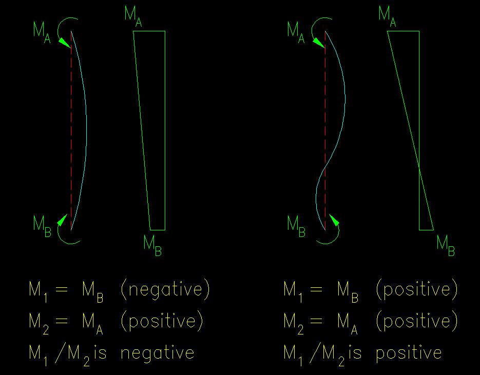
The equation for Cm (SCM equation C2-4) includes terms for the end moments, M1 and M2, which are defined as the smaller (smallest absolute value) and larger end moments, respectively. If, on a free body diagram, the signs are kept true to the right hand rule, the ratio of M1 to M2 will be negative if the member is in single curvature and positive if in reverse curvature as shown in Figure 9.4.1.
Figure 9.4.1
Computation of M1/M2
Click on image for larger view
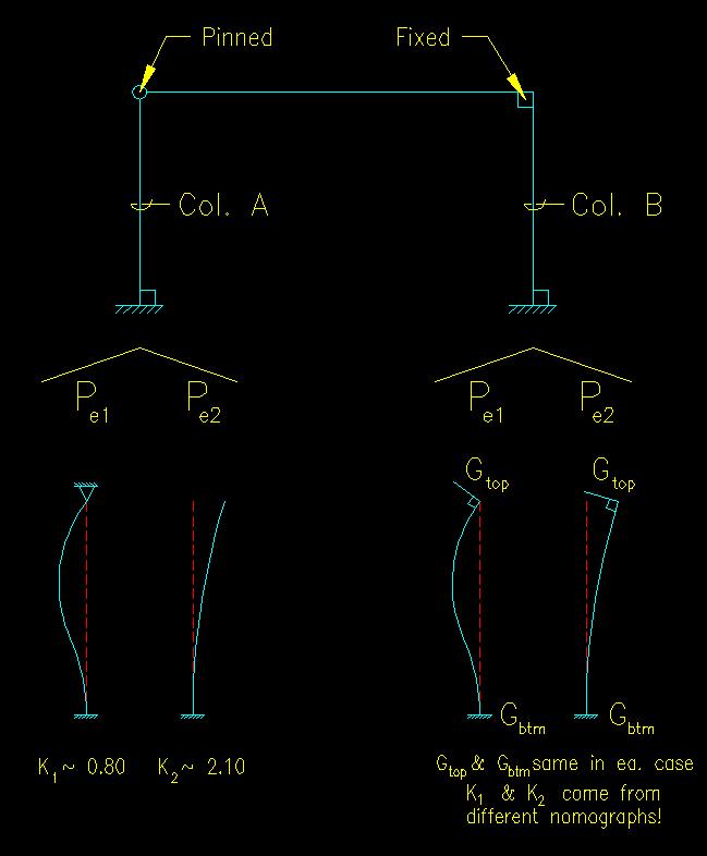
The equations for both B1 and B2 include a term (Pe1 and Pe2) for the Euler buckling load for the column in the plane of buckling/bending that is under consideration. The difference between the two terms is the effective length coefficient, K, used. For Pe1, the value of K used is to assume that there is no joint translation and for Pe2, the value of K used is that for the actual condition. In the case of a column in a braced frame, Pe1 and Pe2 are the same. Figure 9.4.2 illustrates the determination of K1 and K2 for one plane of a frame for two different columns.
Figure 9.4.2
Determination of K1 and K2
Click on image for larger view
In the case of B2, the sum of all the Pr's and Pe2's for all the columns in the frame at the same level is required. This is because all the columns in a frame at the same level have the must move together and have the same joint translation. The combined in-plane bending stiffness of all the columns in the level contribute together to resist lateral motion of the frame in that level. In other words, the story deformation, D, is a function of the bending stiffness of all the columns in the level contributing to lateral stiffness of the structure in the plane under consideration. Consequently the second order effects of all the columns in the level are interrelated.
Again, recall that everything done in these analyses is IN A PLANE. Consequently, when computing the Pe2 for each column, if the column orientations change in the level, some columns Pe2 will be strong axis dependent and some weak axis dependent.
Note that the magnifiers, B1 and B2, are never to be taken as less than 1.00. A value of less than 1.00 suggests that the axial compression reduces the first order moments. This cannot be true, hence the SCM limit on B1 and B2.
Once the magnifiers, B1 and B2, are determined then the axial forces and moments are recombined using SCM equations C2-1 to obtain the required axial force, Pr, and required moments, Mr, for use in the combined force equations.